HENGSHI SENSE Requirements for Data Modeling in Display and Interaction of Tables

For common datasets with large amounts of information, including detailed and summarized types of data concentrated in a single table with a complex format, large information volume, and containing complex statistical operations in the analysis, HENGSHI SENSE provides Chinese-style reports to meet the analysis needs of similar situations, that is, the tables in the HENGSHI system.

Below, using coffee analysis[^1] as an example, we introduce the current HENGSHI SENSE system visualization, the production display, and interaction requirements of the table for the data model.

Introduction to Table Basic Information

The detailed setting of the table is thoroughly introduced in the commonly used section of the chart classification Table, which will not be reiterated here. The main introduction here is the significance of the main items in the table.

Configuration

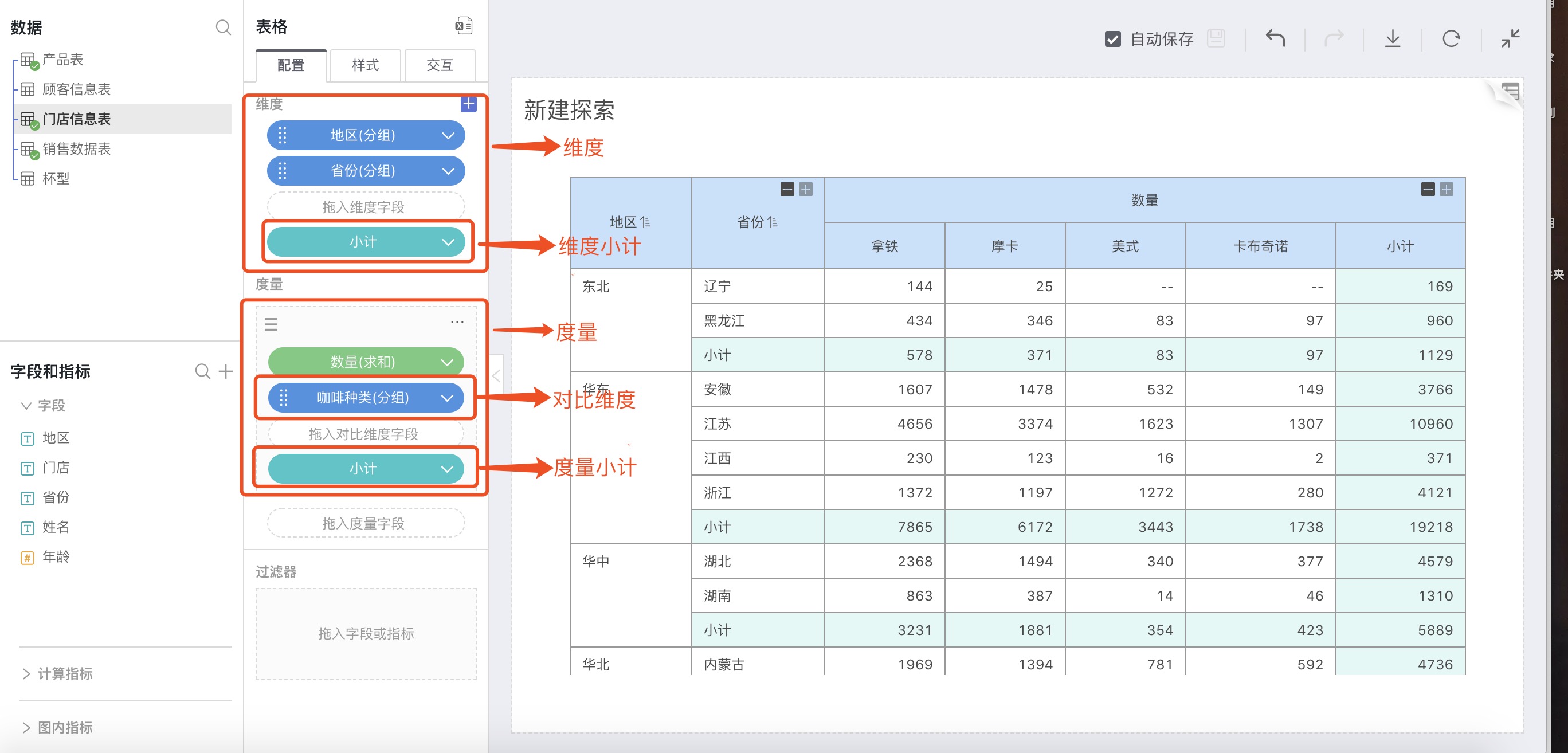
Dimensions

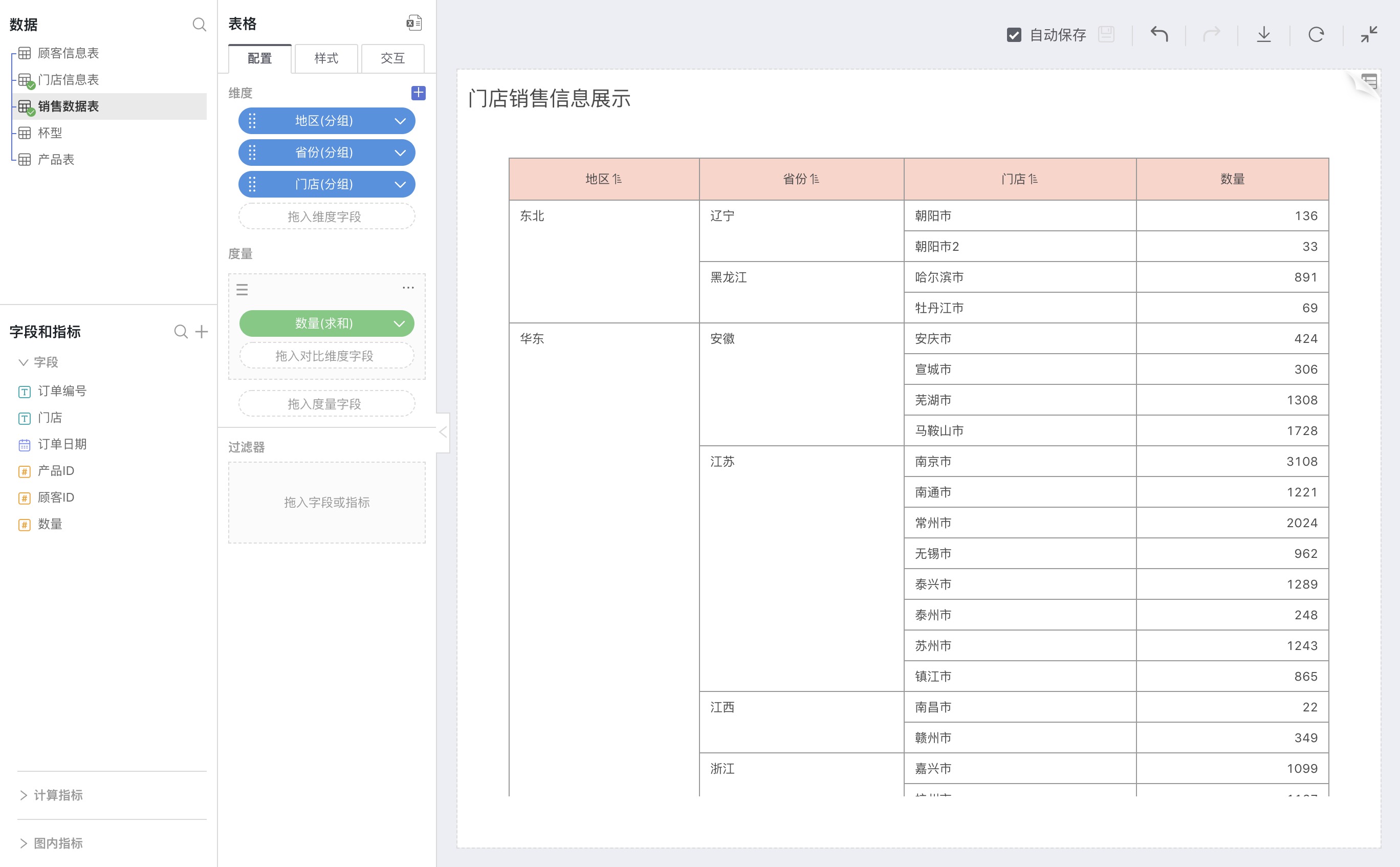
The basis for grouping in visual analysis.

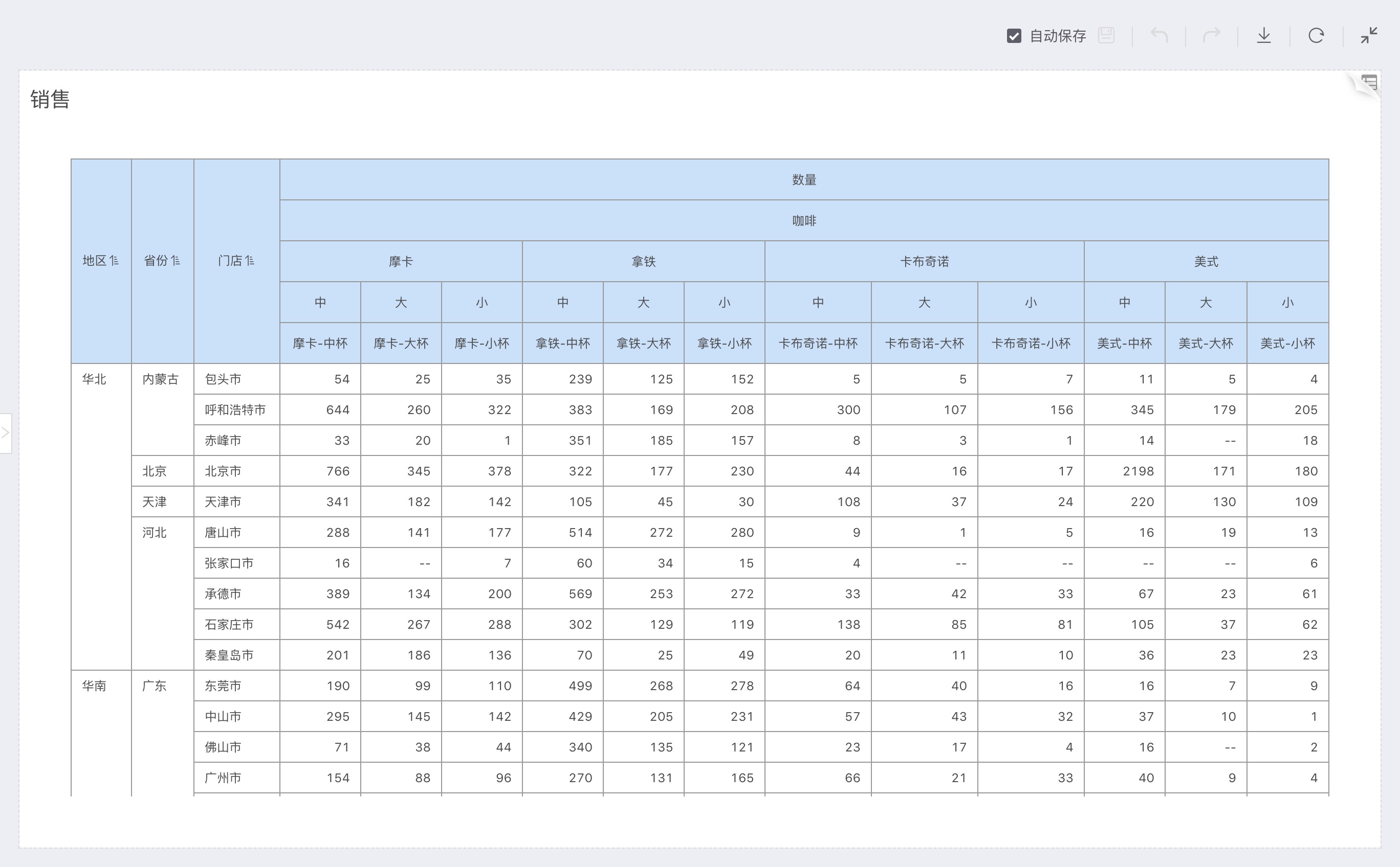
For example: In the above figure, Region and Province are located in the two leftmost columns of the table, grouping data.
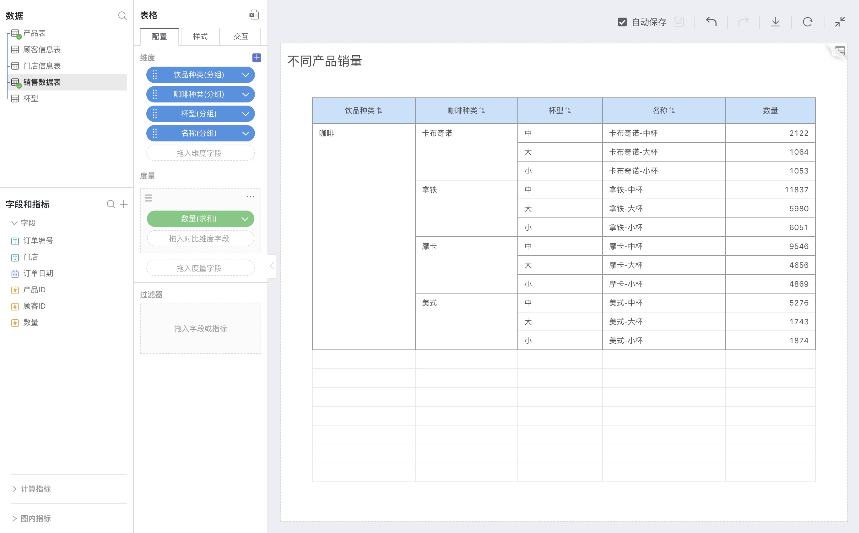
Measures

After grouping by dimensions, the basis for aggregate calculation for each group of data needs to be set.

For example: In the above figure, Quantity is located at the upper right of the table, calculating the sum totals of quantities for each group after grouping by dimensions.
Comparison Dimensions

Comparison dimensions can only be added relative to a single measure, re-grouping the aggregate value of the measure.

For example: In the above figure, the comparison dimension Coffee Type was added beneath the measure Quantity, located below Quantity, re-grouping the values of Quantity, with each group summarizing the calculations separately.
Subtotals for Dimensions

You can select dimensions to add subtotals, grouped by other dimensions, to calculate the sum value in the current dimension, displayed as a row.

For example: In the above figure, the subtotal of dimensions adds a subtotal to dimension Province, then grouped by Region, with each group in Province calculating a summary value.
Subtotals for Measures

You can select comparison dimensions, dimensions to add subtotals, grouped by other dimensions, to calculate the total value in the current dimension, displayed as a column.

For example: In the above figure, the subtotal of measures adds a subtotal for the comparison dimension Coffee Type. At the far right of the comparison dimension column, under measure Quantity, the Quantity values aggregated after grouping by Coffee Type are summed again.

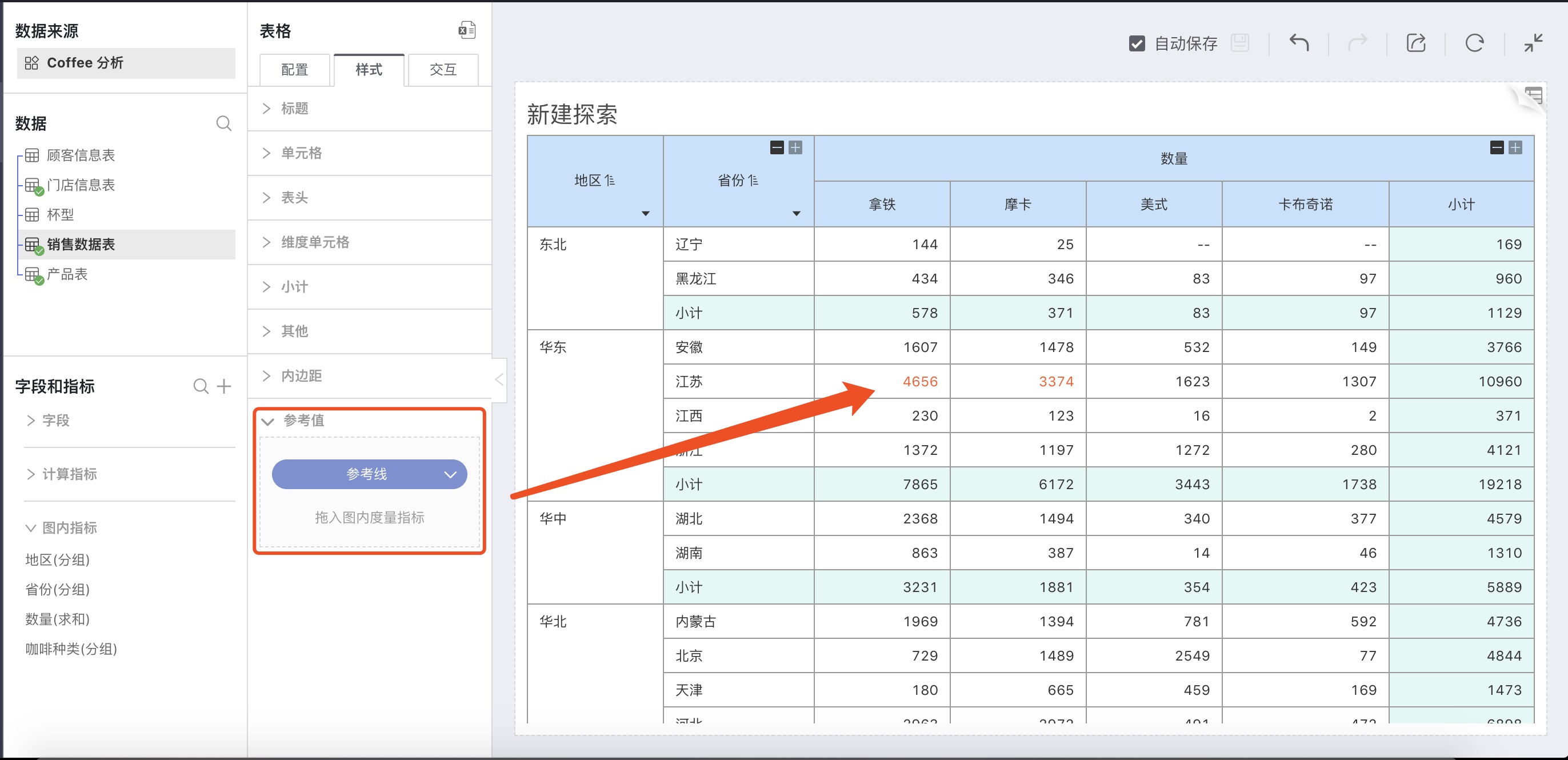
Style

Reference Values

Based on the measure, reference values can be added to mark abnormal data in the chart according to different calculation methods.

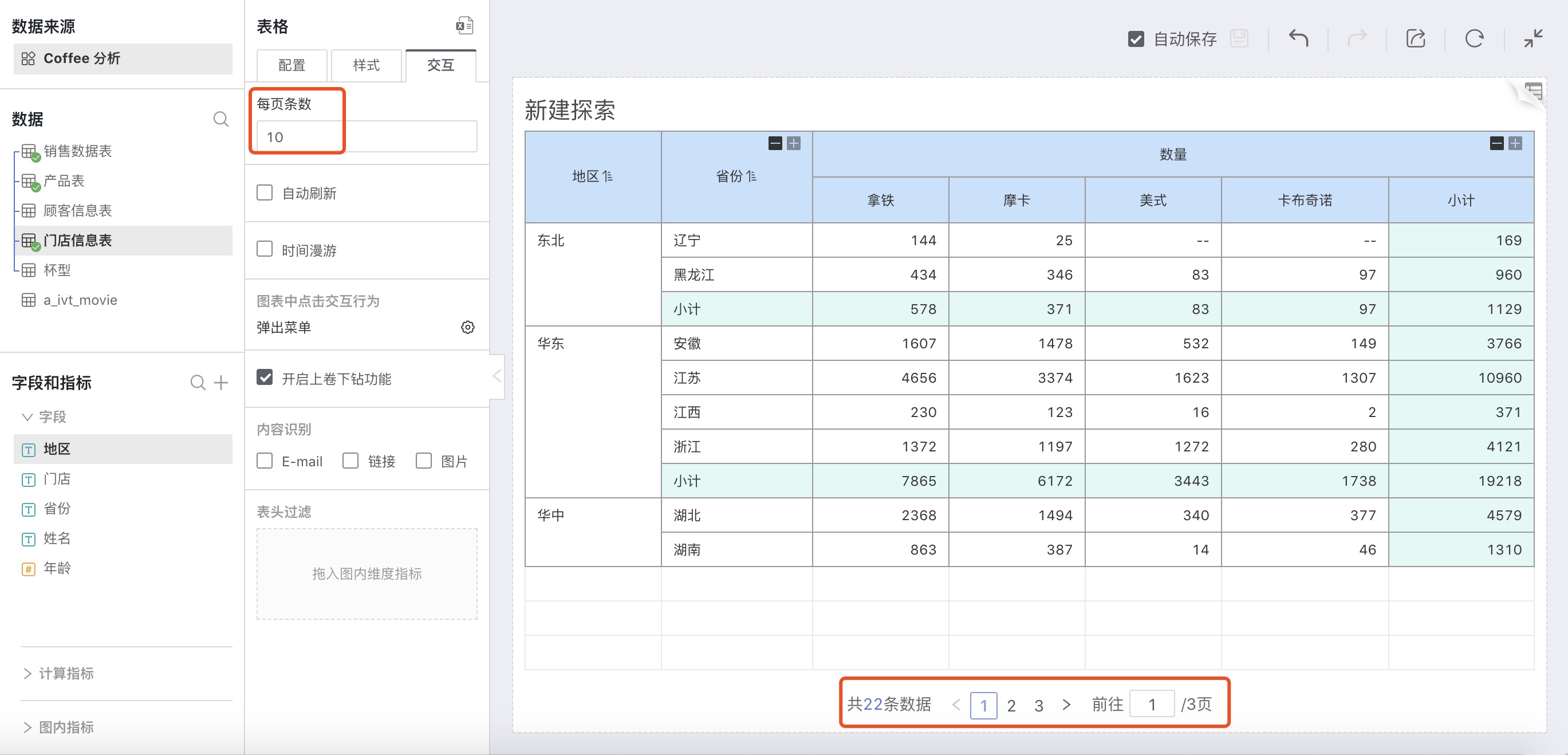
Interaction

Number Per Page

The default is 1000, which can be customized. When the total number of data in the chart is greater than the set number per page, it will be displayed in pages.
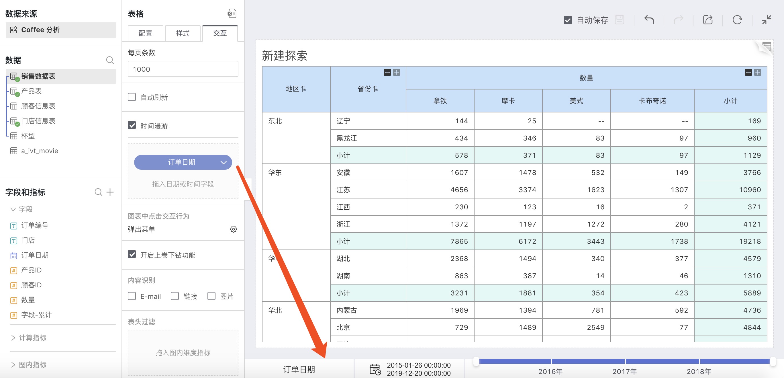
Time Travel

The default is off. After checking, you can drag the date field into the box under time travel, and a timeline will appear at the bottom of the chart, convenient for dragging to view data within different time ranges. The specific operation method is described in detailed in the [Time Travel](chart.md#Time Travel) section.
Enable Drill Up/Down Feature

Checking on the Enable Drill Up/Down feature allows you to start collapsing dimensions/comparison dimensions from the bottom layer, achieving the display of summarizing upwards and grouping downwards. Specific operation as shown below:
Content Recognition

The default is unchecked and can be manually changed, including E-mail, links, images. After checking, the types of columns in the table are automatically recognized, for instance:
1. Link: After checking, the link can be clicked to jump to the corresponding website.
2. Image: After checking, the image can be displayed in the table.
Header Filters

From the left-hand chart indicator grouping, add dimension fields to the header filter. You can temporarily filter and analyze the dimension grouping.

After dragging the dimension field to the header filter, there is a downward triangle at the bottom right of the field name in the header row of the table. Click to expand, list all groups for temporary filtering:

The introduction of table basic information is shown above. Next, we will introduce scenarios suitable for analysis with tables and the requirements of table display and interaction for data models.

Expected Visualization Effects

Analysis Needs

Taking coffee analysis as an example, the study focuses on the sales situation of different products in stores in various regions, as well as the aggregated sales situation at different granularities. Mainly consider the following two factors:

Product Structure: Coffee level information

Various beverages under different drink types are further subdivided into different cup types, and specific products under each cup type.
Store Structure: Store level information

Different stores in different provinces of various regions

Based on the above focus factors, the specific analysis needs are:

Display of product structure and store structure at different levels
Display of product structure and department structure can be summarized upwards and grouped downwards by level.

Expected Effects

From the introduction of basic table information in the first chapter, HENGSHI SENSE provides dimension and comparison dimension for two types of grouping information. Therefore, in the sales analysis, the dimensions and comparison dimensions support the cross-analysis of products and stores. The drill-up/drill-down feature supports analyzing data summarized at product and store level structure and detailed data viewed downwards.

Store level as dimensions, product level as comparison dimensions:
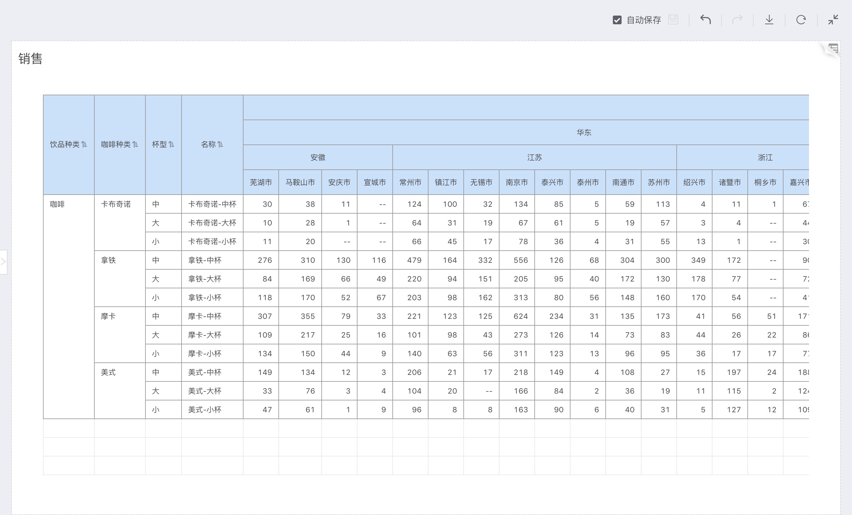
Product level as dimensions, store level as comparison dimensions
Summarize upwards and group downwards according to different granularities

As shown above, for coffee sales in various categories across regions, HENGSHI SENSE can provide two types of table structures:

Department as dimension, product as comparison dimension
Product as dimension, department as comparison dimension

The coffee product structure and store structure have been analyzed to display the needs for subdivision by layer.

By enabling drill-up/drill-down, the analysis needs have been achieved when focusing on granularities at different times, summarizing upwards, and grouping downwards.

However, to achieve the above effects, namely the department level and product level as dimensions and comparison dimensions, the table currently has certain requirements for the data model.

Table-Adapted Data Model

The coffee analysis data is stored across multiple tables, which is closer to customer scenarios, such as sales data belonging to the sales department and product data belonging to the product department.

Product Table

The product table contains detailed information about each product, which category it belongs to at each level of the product structure tree.

Product ID	Drink Type	Coffee Type	Cup Size	Product Name	Price
1001	Coffee	Americano	Large	Americano-L	30
2002	Coffee	Americano	Small	Americano-S	25
3009	Coffee	Latte	Medium	Latte-M	32

For example, 1001, the information on the product structure tree is:

Level1	Level2	Level3	Level4
Coffee	Americano	Large	Americano-L

It's necessary to identify each product's grouping at different levels in order to perform a data analysis in the table where the product serves as a dimension or comparison dimension, open by layer. As shown in the figure below:

Store Information Table

The store information table contains detailed information about the store, and the belonging situation of the store at each level of the store structure tree.

Store	Name	Province	Region
Hangzhou	Lisi	Zhejiang	East China
Chengde	Zhaoliu	Hebei	North China
Mudanjiang	Wangwu	Heilongjiang	North China

For example, Hangzhou, the information on the department structure tree is:

Level1	Level2	Level3
East China	Zhejiang	Hangzhou

It's also essential to identify each store's grouping at different levels of the store structure tree so that we can display the data in the table by expanding the department layer by layer. As shown below:

Sales Table

The sales table breaks down each order into multiple entries according to different product types, each entry corresponding to one type of product in each order. Mainly for statistical calculation of the sales situation for each product, as shown in the table below:

Order Number	Order Date	Store	Product ID	Customer ID	Quantity
20000002	2020-01-01	Beijing	3001	126	5
20000002	2020-01-01	Tianjin	3003	126	6
20000002	2020-02-10	Xi'an	3009	100	2

The table structures are as described above, and we need to aggregate the data information into a single wide table to employ sales data, store, and product in the same table for analysis during visualization. This can be achieved through Multiple Table Joint and Data Model to summarize the data information.

We recommend using data models, which generate a virtual wide table. Compared to the multi-table joint method, where a dataset is established for each analysis, the data model offers greater flexibility and agility for data analysis: edit the relationship in the model at any time, new model relationships can immediately affect the analysis results.

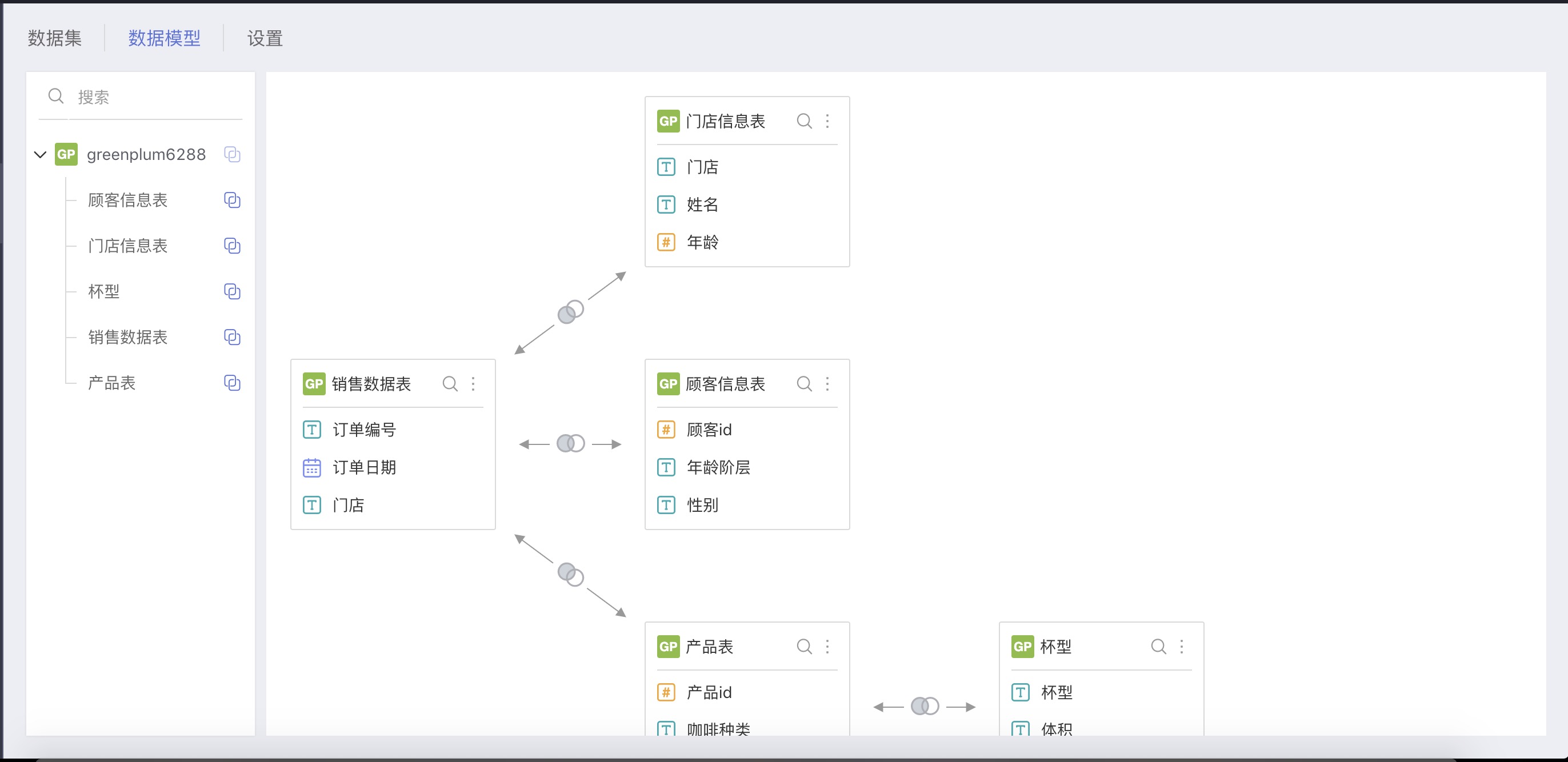
After establishing the data model, you can complete the analysis with the product level and department level as dimensions and comparison dimensions, respectively.

Special Data Structures

Some enterprises' data is not stored in the form mentioned above, but through indexing by product/department level relationships. The difference in storage methods leads to complexity in data processing.

Data Structure

If your enterprise's database stores product and department data indexed by level relationships. Taking the department structure for example, the department relationship is stored indexed by Department ID and Parent Department ID:

id	parentid	name
1001	null	East China
2001	1001	Zhejiang Province
3001	2001	Hangzhou

Each record of sales data records the department ID and the quantity:

date	codename	code id	amount
20200107	Hangzhou	3001	3
20200109	Hangzhou	3001	5

With the above data structure, to adapt the table for data analysis in visualization, you need to preprocess the data at the bottom level before entering it into HENGSHI SENSE.

Data Processing Before Entering HENGSHI SENSE

As aforementioned, data schema format:

All stores are in a tree structure, with each store's position on the store structure tree recorded through ID and ParentID. It is necessary to use the corresponding IDs and ParentIDs to unfold the indexed structure storage table into a flat level structure table, sorting out the hierarchical relationship of the stores.

For example: In the third layer of the tree structure, the specific information for each store, such as Hangzhou, needs to be integrated into the third-level classification. Hangzhou's province is Zhejiang, which needs to be integrated into the second-level classification.

This preparation enables us to display department information in the table layered in later visualization.

The processed table structure is shown below:

code id	Level 3	Level 2	Level 1
3001	Hangzhou	Zhejiang	East China

Note

Footnote 1: The data and analysis scenario of coffee analysis are described in detail in Advanced Computing Usage Instructions.